Imagine you stumble into a medical conference and decide you want to socialize with physicians. Your process may be to approach a random physician, speak to them for a bit, and then have them randomly select one of their colleagues whom you can speak to next. If you continued like this forever, how much time would you spend talking to each person? You might spend the most time talking with the person with the most connections, but depending on how the data is structured, that might not be the case. Let's take a look!
Step 1: Get a hold of the data you want to analyze and format it as an edge list in a csv. An edge list has two columns which both represent nodes in the graph. For example, a row like 103, 105 might represent that physician 103 is connected to physician 105.
Step 2: Install R, as well as the igraph package.
Step 3: Build a graph with the igraph package from your csv edge list. Running the function below prompts the user to select a csv file from the system and builds a graph.
library(igraph)
graphFromEdgeList <- function(){
  dat=read.csv(file.choose(),header=TRUE) # choose an edgelist in .csv file format
  graph.data.frame(dat,directed=TRUE)
}
Step 4: Manipulate the graph using some of the techniques from Google's page rank paper and build a transition matrix.
Before moving to step 5, let's take a quick look at graph theory. An adjacency matrix is a representation of a graph where a spot in the matrix (for example, [103,105]) is 1 if physician 103 is connected to 105, and 0 if they aren't connected. To get the probability of randomly transitioning from any given node to any of its connections, you divide 1 by the number of connections for the physician. If physician 103 has 5 connections, then there would be a 1/5 or .20 chance of physician 103 directing you to 105. A matrix of all these probabilities is called a transition matrix.
But what happens if physician 103 is connected to 104 but 104 is connected to nobody? Or what if 104 is only connected to 105 and 105 is only connected to 104? These two examples, also known as leafs and periodic subgraphs, can distort the results of a random walk because the walker could never get to the rest of the graph. When Google was working on its page rank algorithm they came up with some tricks to ensure that the graph they analyzed would not have either of these properties. First, if a node has no outbound connections, then connect it to everything in the graph at equal probability. Second, the walker is given a 20% chance of jumping to anyone randomly at any time. The code to build such a transition matrix given a graph object is below:
# takes a weighted & directed graph
# returns a modified n x n transition matrix
  # return matrix is modified so that any node that had no outbound edges is
  # connected to every node in the graph at a uniform weight.
  # Every node is connected so the graph is guaranteed not to have hidden periodic graphs
randomChatterMatrix <- function(G){
  A <- get.adjacency(G) # warning this matrix can be quite large
  N <- nrow(A)
  r <- c()

  for (i in 1:N){
    s = sum(A[i,])

    if (s == 0){
      # connect all leafs to every other node in the graph at equal probability
      # manipulating A in a loop is not performant because it will copy A every time
      # keep a vector of rows to bulk update later
      r = c(r, i)
    } else {
      # since s varies row to row perform the operation on the spot
      A[i, ] <- A[i, ] / s
    }
  }

  A[r,] <- 1/N # bulk update all zero rows
  m <- as.matrix(A)
  (.8 * m) + (.2 * 1/N)
}
Step 5: Compute the random walk probabilities for each physician. Now that we have a transition matrix to work with, we can use linear algebra to answer our original question. How much time will you spend talking to each person? It just so happens that when you're dealing with a real square matrix with positive entities, the eigenvector corresponding to its largest eigenvalue will give us exactly that information. Using the functions above the code to compute the dominant eigenvector looks like this:
g <- graphFromEdgeList()
r <- randomChatterMatrix(g)
eigen_vect = eigen(t(r))$vectors[,1]
probs = eigen_vect/sum(eigen_vect)
print(probs) # lets see what we got!
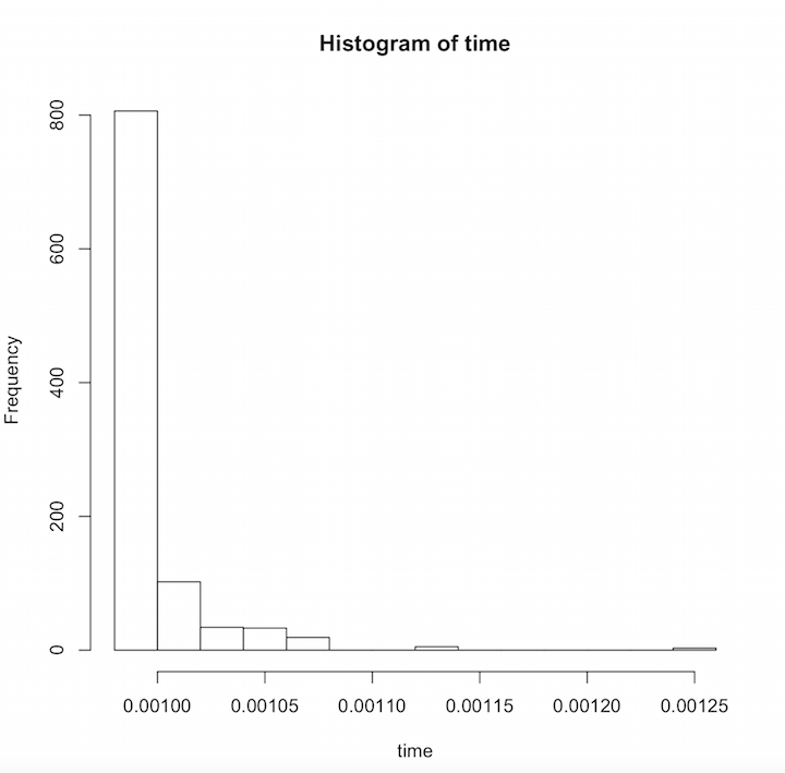
Below is a graph of a small subset of Doximity physicians where the X axis shows the proportion of time spent talking to a physician and the Y axis shows how many physicians fell into that amount of time. The results follow a logarithmic trend where you would randomly chat with most physicians for about the same amount of time. A few physicians however stand out as people you would spend significantly more time chatting with.

And just like that, you're able to quantify exactly how much time you would spend with each physician. This new piece of information is interesting on its own, but it can also be the start of many more fun data science exercises with R!
